

This is a description of how we usually calculate the uncertainties of concentrations and ages and some practical examples on cosmonuclide analysis.
Theory
Considering that
- All operators (e.g. analytical data) are well represented by normal distributions.
- We are considering uncertainties of independent variables (no covariance).
- The uncertainty of the result is small enough to be well represented by a normal distribution. This means that the result is roughly linear in the area of the uncertainty and therefore the resulting distribution is not asymmetrical.
the error propagation should be performed by considering the partial derivatives of the result respect the operators:

where 

Examples of common operations
| Operation | Formula | Uncertainty |
| General |  |  |
| Addition |  |  |
| Subtraction |  | |
| Multiplication |  |  |
| Division |  |  |
| Power |  | 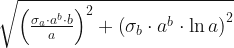 |
| Natural logarithm |  | 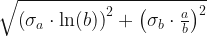 |
| Logarithm to base 10 |  |  |
Examples applied to cosmogenic isotope data
Calculating a 10Be age
The apparent 10Be age t of a surface sample with a 10Be concentration of C is
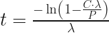
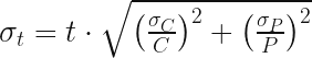
where P is the production rate and λ is the radioactive decay constant. According to the general equation, the uncertainty of the apparent age σt should be calculated as

where σC and σP are the uncertainties of the concentration and the production rate, respectively. However, as 

26Al/10Be burial age
If we calculate a 26Al/10Be burial age t as
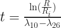
where R is the 26Al/10Be ratio, Ri is the initial ratio, λ10 and λ26 are the radioactive decay constants, and σR and σRi are the considered independent one-sigma uncertainties, the error of the burial age should be:

In this case, this equation is often not realistic because the previous equation does not fit the third assumption (asymmetrical error) for typical R uncertainties from too young (R/Ri>0.8) or too old samples (R/Ri<0.2). Therefore, in this case, it is highly recommendable to calculate the extreme values of t (t+σt and t–σt) by varying the burial equation as follows:

to check the asymmetry and, if necessary, calculate the positive and negative errors of t (t+σt and t–σt) from the maximum and minimum values obtained from the last equations.
Calculating a 21Ne concentration
If we consider that a cosmogenic 21Ne concentration is calculated as:
![[^{21}Ne] = \frac{\left( R_{Sample}-R_{Air} \right) \cdot N_{20}}{M}](https://s0.wp.com/latex.php?latex=%5B%5E%7B21%7DNe%5D+%3D+%5Cfrac%7B%5Cleft%28+R_%7BSample%7D-R_%7BAir%7D+%5Cright%29+%5Ccdot+N_%7B20%7D%7D%7BM%7D&bg=ffffff&fg=111111&s=3&c=20201002)
where R are the measured 21Ne/20Ne ratios, N20 is the total number of 20Ne atoms, M is the mass of the sample and we are considering σRSample and σN20 as independent errors, the uncertainty of the 21Ne concentration should be
![\sigma_{[^{21}Ne]} = \sqrt{\left( \frac{\sigma_{RSample} \cdot N_{20}}{M} \right) ^2 + \left( \frac{\sigma_{N20} \cdot (R_{Sample}-R_{Air})}{M} \right) ^2}](https://s0.wp.com/latex.php?latex=%5Csigma_%7B%5B%5E%7B21%7DNe%5D%7D+%3D+%5Csqrt%7B%5Cleft%28+%5Cfrac%7B%5Csigma_%7BRSample%7D+%5Ccdot+N_%7B20%7D%7D%7BM%7D+%5Cright%29+%5E2+%2B+%5Cleft%28+%5Cfrac%7B%5Csigma_%7BN20%7D+%5Ccdot+%28R_%7BSample%7D-R_%7BAir%7D%29%7D%7BM%7D+%5Cright%29+%5E2%7D&bg=ffffff&fg=111111&s=3&c=20201002)
that can be also expressed as
![\sigma_{[^{21}Ne]} = [^{21}Ne] \cdot \sqrt{\left( \frac{\sigma_{RSample}}{R_{Sample}-R_{Air}} \right) ^2 + \left( \frac{\sigma_{N20}}{N_{20}} \right) ^2 }](https://s0.wp.com/latex.php?latex=%5Csigma_%7B%5B%5E%7B21%7DNe%5D%7D+%3D+%5B%5E%7B21%7DNe%5D+%5Ccdot+%5Csqrt%7B%5Cleft%28+%5Cfrac%7B%5Csigma_%7BRSample%7D%7D%7BR_%7BSample%7D-R_%7BAir%7D%7D+%5Cright%29+%5E2+%2B+%5Cleft%28+%5Cfrac%7B%5Csigma_%7BN20%7D%7D%7BN_%7B20%7D%7D+%5Cright%29+%5E2+%7D&bg=ffffff&fg=111111&s=3&c=20201002)
and it is always larger than
![{[^{21}Ne] \cdot \sqrt{\left( \frac{\sigma_{RSample}}{R_{Sample}} \right) ^2 + \left( \frac{\sigma_{N20}}{N_{20}} \right) ^2 }} \quad \neq \quad \sigma_{[^{21}Ne]}](https://s0.wp.com/latex.php?latex=%7B%5B%5E%7B21%7DNe%5D+%5Ccdot+%5Csqrt%7B%5Cleft%28+%5Cfrac%7B%5Csigma_%7BRSample%7D%7D%7BR_%7BSample%7D%7D+%5Cright%29+%5E2+%2B+%5Cleft%28+%5Cfrac%7B%5Csigma_%7BN20%7D%7D%7BN_%7B20%7D%7D+%5Cright%29+%5E2+%7D%7D+%5Cquad+%5Cneq+%5Cquad+%5Csigma_%7B%5B%5E%7B21%7DNe%5D%7D&bg=ffffff&fg=111111&s=3&c=20201002)
which is not a realistic way of calculating the uncertainty of [21Ne] unless RSample>>RAir. Also, for samples where RSample values are close to RAir, the uncertainty of [21Ne] might be asymmetrical, and it is highly recommendable to check the shape of the [21Ne] uncertainty as explained in the burial section.
